Perfect competition (characteristics)

1. Many small independent producers and consumers

• All firms are too small to influence market in any way, hence there are multiple producers in the market

• This means that no 1 firm can drive up or down the prices of the products in the market by influencing the output

• Consumers on the other end can also not influence the prices by consuming more or less

2. Firms produce a standardized product

• All firms in the market produce almost the same product

3. No barriers to entry or exit

• No significant obstacles to the entry of new firms into, or the exit of existing firms out of, this industry

4. Firms are “price takers”

• Since none of the firms can influence the prices, they go along with the prices which are set by the market and produce how much they want

• Any firm which tries to increase the price even by a dollar would end up losing customers, due to as mentioned earlier about the production of standardized products

• Consumers would not prefer buying expensive products if they can get it cheaper elsewhere

Demand for the firm

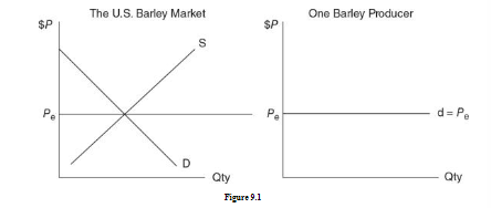
• Since each firm’s output is such a small share of the total market supply, the demand for each firm’s output is perfectly elastic

• They simply produce as much as they can at the going price hence a horizontal demand curve

• Keep in mind that the horizontal demand curve is of individual producers, not the market demand curve

Profit Maximization

• Maximizing economic profit is highest possible difference between total revenue and total economic cost

• Any opportunity is seized where even if one extra dollar is being earned

• If the maximum profit possible is actually zero, or even negative dollars, they accept this short-run outcome

Methods to maximize profits

1. The Method of “Totals’’

• Since prices can’t be altered, firms look to manipulate the output.

• Imagine a carrot farmer operating in a perfectly competitive market, sales carrots for $11

• As noticeable from the chart, total cost increases with increased production

• Logically, the carrot farmer would grow 5 bushels of carrots to generate more economic profit

• When there are two quantities that produce the same amount of profit, like 4 and 5 bushels, we select the larger of the two quantities

2. The Method of “Marginal”

• Only decision to be made by perfectly competitive firm is to choose the optimal level of output.

Decisions are as follows

1. Choose the level of output where MR = MC

2. Since MR=MC at 5 bushels of carrot, the farmer would grow that level

3. Price = Marginal revenue in perfectly competitive market structures

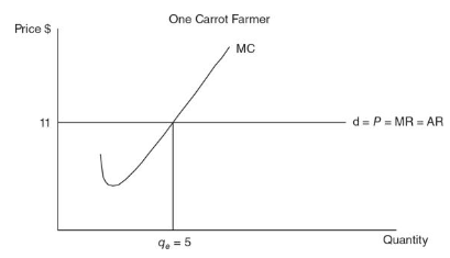
4. This is because Farmers can sell as much as they want at the market price hence earn the same amount of marginal revenue

5. Price is also equivalent to average revenue (AR), or total revenue per unit

Short-run profit and loss

• Profit = qe x (P-ATC)

• The term (P - ATC) is the per-unit difference between what the firms receives from the sale of each unit and the average cost of producing it, or profit per unit

• Multiply this per-unit profit by the number of units (qe) produced, you have total profit

Profit rectangles and flying monkeys

• Never leave this level of output (qe)or bad things happen

• We have positive economic profits of $2 if we produce at qe

Short-run losses

• MR=MC at 3 bushels now, however the carrot farmer would now face economic losses instead

• At this point however, the farmer is able to minimize losses the most at this level

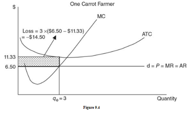
• This becomes the loss minimizing level for him

When finding the profit/loss rectangle, it is important to remember the following:

1. Find qe where P = MR = MC. Once you have found qe, never leave it

2. Find ATC vertically at qe. If you move downward, π > 0. If you move upward, π < 0

3. Move horizontally from ATC to the y-axis to complete the rectangle, and clearly label it as positive or negative

Decision to shut down

• If firms are incurring losses, they must decide whether it is economically rational to operate at all

• Decision to shut down, or produce zero, in the short run is sometimes the optimal strategy

2 things happen when firms produce output > 0

1. Total revenue is generated

2. Total variable cost is incurred (fixed cost is incurred irrespective of output)

   1. If the firm is able to at least meet its total variable cost irrespective of fixed cost, it continues to operate under losses

   2. However if the situation is dire and they are unable to cover their TVC, the firms best choice if to shutdown operation

   3. This strategy would prevent firms from incurring more losses and only take the fixed cost as their losses

   4. If TR ≥ TVC, the firm produces qe where MR = MC.

   5. If TR < TVC, the firm shuts down and q = 0

The shutdown point

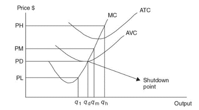
• If P ≥ AVC, the firm produces qe where MR = MC.

• If P < AVC, the firm shuts down and q = 0

• PH is the highest price. At qh, the firm earns enough total revenue to cover all costs (π > 0)

• PM is the middle price. At qm, the firm’s TR exceeds TVC but only covers part of the TFC. π < 0.

• PD is the shutdown price. At qd, the firm’s TR just covers TVC and the firm is at the shutdown point. If price falls any lower, the firm does not produce.

• PL is the lowest price. At q1, the firm’s TR cannot even cover TVC, and so the firm shuts down, producing q = 0. π = -TFC

Short-run supply

• If price increases, quantity supplied increases

• If price decreases, quantity supplied decreases

• When the price falls below the shutdown point (minimum of AVC) and the firm quickly decides to produce nothing

• The MC curve above the shutdown point serves as the supply curve for each perfectly competitive firm.

• The market supply curve is therefore the horizontal sum of all of the MC curves: S = S MC

Long-run adjustment

• Firms enter and leave a perfectly competitive market based on the level of profits being made or the incurring of losses

Short-run positive profits

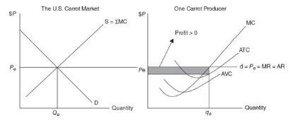
• Since the market price is above ATC, the firms in the market are earning a short term profit

• In the long run however, seeing the success of the firms in the market, more firms join in

• As more firms join in, the supply gradually increases because of which the market price comes down

• As the market price comes down, firms already in the market begin to make less and less profit until there is no profit at all

• At the point where P = MR = MC = ATC, each carrot farmer is now breaking even with π = 0

• This breakeven point is described as the long-run equilibrium

• Market quantity increases and Individual producer output falls.

What’s so great about breaking even?

• Economic profit subtracts the next best opportunity costs of your resources from total revenue

• Accounting profit is simply total cost – total revenue

• You are making a fair rate of return on your invested resources and you have no incentive to take them elsewhere

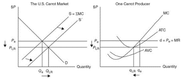
Short-run losses

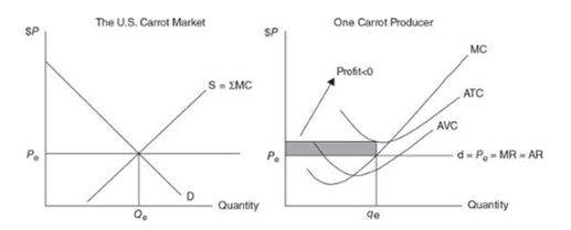
• Since market price is below ATC, the firms in the market incur losses

• In the long run, when firms continue to incur losses, most of them would begin to leave the market

• As more firms leave, the supply would automatically cut short, raising the market price

• Overtime, losses would be reduced further leading to breaking even point eventually

• At the point where PLR = MR = MC = ATC, each remaining carrot farmer is now breaking even with π = 0

• Market quantity decreases and Individual producer output rises.

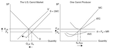
Conclusion

• All the assumptions made up till now rely on one more assumption which is that it’s a constant cost industry

• When new firms enter markets, the demand for key resources increases which in return increases the cost that would be incurred to employ these

• The cost curves for firms in the industry start to shift upward and this is known as increasing cost industry

• Entry of new firms drives down the price of the output and increases the cost curves, so the profit is eliminated more quickly than with our constant cost industry

• Fewer firms eventually enter and the new long-run price is higher than it is in a constant cost industry

• A decreasing cost industry is one in which the entry of new firms decreases the price of key resources and causes the cost curves to shift downward

• The entry of new firms lowers the price of the output and decreases the cost curves, it takes longer for the profit to be eliminated than in our constant cost industry

• More firms can eventually enter this market, and the new long-run price is lower than it would be in a constant cost industry

Monopoly (characteristics)

1. A single producer

   1. No firms in industry at all

2. No close substitutes

   1. Since only one firm dominates, there aren’t any substitutes available

3. Barriers to entry

   1. Very high barriers to entry which prevents competition and limits consumer choice

4. Market power

   1. Combining all factors above, monopolist dominate the market with their power

Barriers to entry

1. Legal barriers:

• A benefit of any sort, provided solely to one firm only

• This could be in the form of suppose being the only firm allowed to market their ads or being the only firm, which the government has allowed to sell in the market

• Intellectual properties such as patent or trademarks also help in formation of monopoly to an extent

2. Economies of scale:

• Cost advantage which is received due to fall in average cost as firm grow big in size, in the long run

• Extensive economies of scale by a firm lead to industry relying on them solely

• Natural monopoly are where economies of scale are so extensive that it is less costly for one firm to supply the entire range of demand e.g. power plants

3. Control of key resources

• Control of major resources by one firm makes it very difficult for other firms to enter and produce in the market

Monopoly demand

• Monopolist have to pay attention to law of demand

1. Demand, Price, and Marginal Revenue

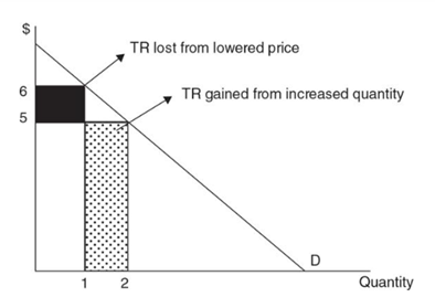
• Price > marginal revenue because the monopolist must lower price to boost sales

• Added revenue from selling one more unit is the price of the last unit less the sum of the price cuts that must be taken on all prior units of output

• Demand is elastic above the midpoint of a linear demand curve, hence price decrease increases total revenue

• Demand is inelastic below the midpoint, hence price decrease decreases total revenue

• Total revenue is maximized at the midpoint and demand here is unit elastic

• Monopolists would avoid the inelastic portion of the demand curve and produce somewhere left of the midpoint

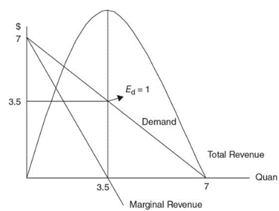
• As visible from the curve, marginal revenue is zero when total revenue is maximized

• Further price cuts decrease total revenue, making marginal revenue negative

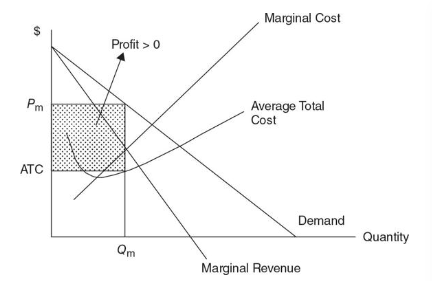
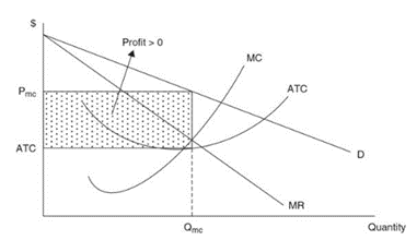
Profit maximization

• The firm must set output at the level where MR = MC. At this level of output (Qm), the monopolist sets the price (Pm) from the demand curve

• Monopoly profits are due to the entry barrier, to last into the long run

• Incase demand plummets or perhaps production costs increase, to the point where P < ATC and losses are incurred, monopolist would leave the market if situation continues

Efficiency Analysis

• Allocative efficiency is achieved when the market produces a level of output where the marginal cost (MC) to society exactly equals the marginal benefit (P) received by society

• Total welfare is maximized at that level and any movement from the output would result in deadweight losses

• Productive efficiency is achieved if society has produced a level of output with the lowest possible cost

• In perfect competition, allocative efficiency is achieved in the long run where P = MR = MC at Q

• Productive efficiency is achieved because firms produce at minimum ATC, once entry or exit has occurred in the long term

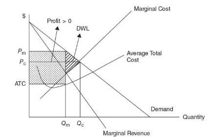
• Monopoly doesn’t have both of these

• Monopolist produces at a quantity Qm where Pm > MR = MC

• This indicates that monopolists purposely don’t produce more, even though demand is there

• This is known as market failure

• The monopoly output isn’t at point where ATC is minimized;

• This explains why monopolist aren’t productively efficient

• A profit earned by the monopolist is a transfer of consumer surplus from consumers to the firm

Price discrimination

• It is the selling of the same good at different prices to different consumers e.g. Airline companies use this strategy

Successful price discrimination is possible if three conditions exist

1. Firm has price control

2. Firm is able to identify and separate groups of consumers e.g. high and low income consumers

3. Firm is able to prevent resale between consumers (make sure the next consumers doesn’t get to know about the discrimination)

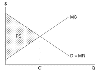
Perfect price discrimination

• This occurs when the firm is able to charge the maximum possible price from different consumers for the same product

• Imagine a scenario where a shop has a system that displays the maximum price each of their customer entering could pay for that product

• This maximum price is easily visible to the cashier only and not to the consumer

• For each different consumer, the maximum price they could pay would vary and the cashier would charge them that exact maximum price they can afford

• The demand curve and marginal revenue are now the same (P = MR) for this

• No single equilibrium price, because each customer was charged a different price

• The monopolist takes all of it as producer surplus since there isn’t any consumer surplus

• Last unit sold is the one for which P = MC, this outcome is allocatively efficient

Monopolistic competition (structure)

1. Relatively large number of firms

• There aren’t countless number of firms like perfect competition but there are quite a few number of firms each with a little market share

2. Differentiated products

• This feature differs them from perfectly competitive firms

• This allows them to set price above competition level

3. Easy entry and exit

• Few barriers and the greatest one perhaps is that of marketing to showcase your differentiated product

Short-run profit maximization

• Just like in a monopoly, demand curve is downward sloping due to their differentiated product

• Similar substitutes available to consumers makes demand quite elastic

• the firm sets Qmc where MR = MC and sets the price from the demand curve

Long-run adjustment

• Since easy entry and exit are there, profits aren’t going to be there in the long run

• New firms entry into industry causes the market share of all existing firms to fall

• As the price begins to fall, the profit reduces

• Monopolistically competitive firms typically engage in extensive advertising to slow down, and even reverse, declining market share

• This however is a short term effect

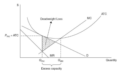
Efficiency and excess capacity

• In long-run monopolistic competition, the firm earns normal profit of 0

• P > MR = MC, allocative efficiency is not achieved due to the differentiated products

• Breakeven level is achieved but the firms aren’t running on minimum ATC, hence productive efficiency isn’t achieved too

• Monopolistic competition output Qmc - output at minimum ATC = excess capacity

• It involves producing at an output less than that which minimizes ATC, hence the assets of the firm are underutilized

• Market is overpopulated with firms, each producing enough to break even in the long run, but so many firms means that each produces below full capacity

Oligopoly (structure)

1. A few large producers

• Distribution of market share in an industry is among few large firms only

2. Differentiated or standardized product

• Oligopoly has a combination of both kind of products

3. Entry barriers exist

4. Mutual interdependence

• The action of one firm (price setting or advertising) is likely to affect the others and prompt a response

Industry concentration

• Sum up the market share of the top 4, or 8, or 12 firms and create a concentration ratio

• If the top 4 firms have a combined ratio of 85% (this is not universally agreed value as some economist prefer even 40%), the market is considered to be oligopolistic

Game theory and the prisoner’s dilemma

• Imagine a case where a two-firm oligopoly (a duopoly) engages in a daily pricing decision

• Each firm knows that if it sets a price higher than the rival’s, it loses sales

• Likewise, if it sets a price below the rival’s, it steals sales

• This non-collusive model of pricing is called the prisoner’s dilemma

Example

• A college professor suspects two students (Jack and Diane) of cheating on a take-home final exam, but she cannot prove the guilt with enough certainty to fail both students in the course or expel them from the school

• The college professor comes up with the following agreement which he discusses with each student individually

• From the above payoff matrix (chart above), it becomes clear that Dianna’s best strategy should be to confess

  • Whether jack confesses or not, Dianna would benefit the most in both scenarios by confessing

  • If Jack confesses, Dianna simply fails the course instead of getting expelled if she too confesses

  • If jack decides to stay silent, Dianna gets a better grade if she confesses

  • Confession hence becomes her dominant strategy

Conclusion

• Outcome of the game is the Nash Equilibrium (if both confess)

• In term of economics, if each player’s strategy maximizes his or her payoff, given the strategies used by the rival players, this is the Nash Equilibrium

• This is a dilemma because if Jack and Diane could only agree to give the professor the silent treatment, they would both walk away with a D, which is better than failing the course or expulsion

• Without such a binding agreement, cheating on the pact would be quite tempting, maybe even fairly predictable

Is every game a prisoner’s dilemma?

• Suppose there are two hamburger stands in town, Stinky’s and Sloppy’s, and each firm sells what it considers to be the best burger in town

• Both burger stands are considering a move to offer hot dogs on the menu, or they could do nothing and continue to offer only burgers

• Stinky’s has a dominant strategy of adding hot dogs to the menu while sloppy doesn’t have any

• Sloppy’s recognizes that Stinky’s is going to add hot dogs to the menu and will respond by maintaining a burgers-only menu

• The Nash equilibrium combination of payoffs is $600 for Stinky’s and $200 for Sloppy’s

• No alternative outcome that would, with prior collusion, increase profits for both firms and hence this isn’t a prisoner dilemma situation

Collusive pricing

• Explicit collusive behavior between direct competitors is an illegal business practice but does occur in the form of tacit (understood collusion)

• Two competitors over time figure out that repeated attempts to undercut the price of their rivals is counterproductive

• Hence if both set the price high, both firms win

• When one cheats on this “understanding,” the other inflicts punishment with a retaliatory price cut

Cartels

• Cartels are groups of firms that create a formal agreement not to compete with each other on the basis of price, production, or other competitive dimensions

• Cartels are more organized forms of collusive oligopoly behavior

• They collectively operate as a monopolist to maximize their joint profits

• Each cartel member agrees to a limited level of output resulting in a higher cartel price

• Joint profits are maximized and distributed to each member

Challenges faced by cartels

1. Difficulty in arriving at a mutually acceptable agreement to restrict output

2. Punishment mechanism

   1. cartel members have the incentive to cheat by producing more than their allotment

3. Entry of new firms

   1. Entry of new firms lead to cartel’s losing their monopoly power and profit.