
Unit 3 - Production, Cost, and the Perfect Competition Model Guide
3.1 - The Production Function
Production function : relation between the quantity of inputs a firm uses and the quantity of output it produces.
Also related to how firms produce goods using the factors of production (land, labor, capital, and entrepreneurship)
Some terms you will encounter a lot:
Fixed input : an input whose quantity doesn’t change
Variable input : an input whose quantity can change
Long run : time period in which all inputs can be variable
Short run : time period in which at least 1 input is fixed
Marginal product : change in overall output when input changes
Marginal product of labor (MPL) : ∆Q/∆L
Diminishing marginal returns : as input increases, the output of each input will be less than the previous input
Output : quantity produced
Rental rate : price of capital
Capital : goods that are used to produce goods/services
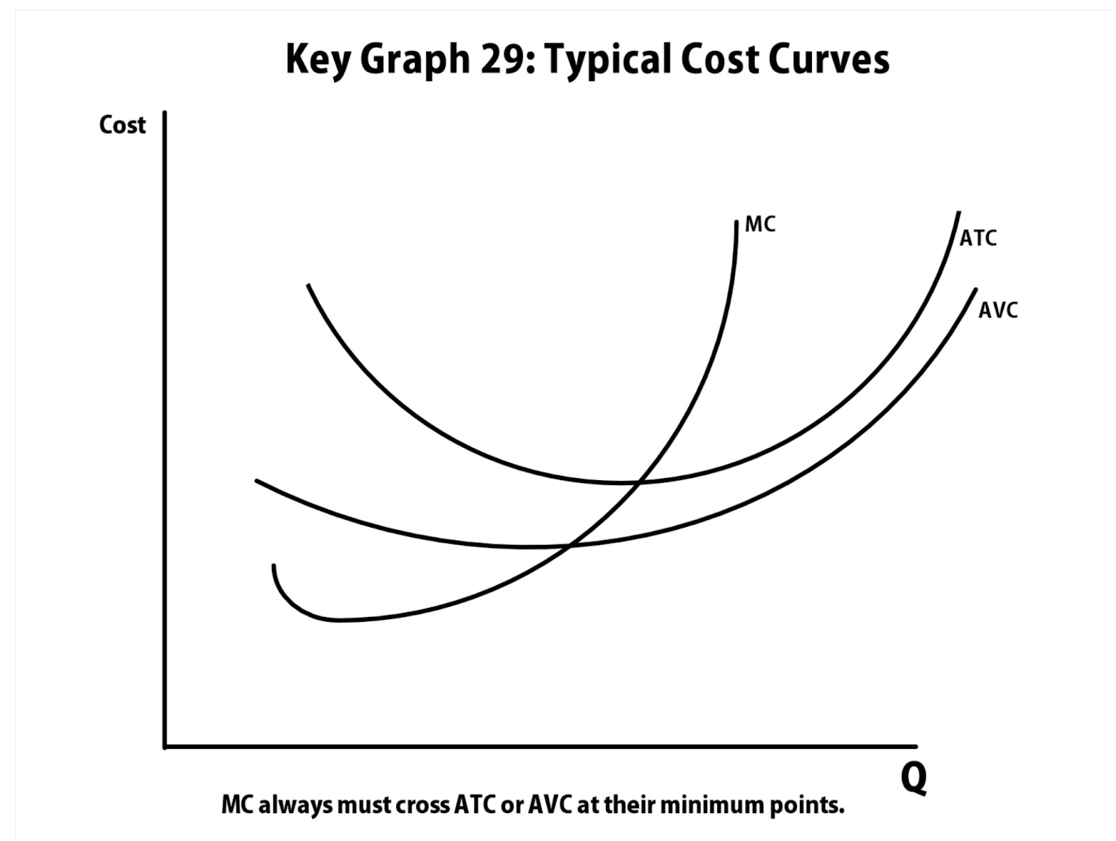
3.2 - Short-Run Production Costs
This portion aims to look into how costs change depending on quantity in the short run. The short run is the period in which at least one of our inputs are fixed. On the other hand, the long run looks into costs which aim to minimise our costs.
This can be measured by understanding the following concepts
Fixed cost : cost that doesn’t change with amount of output produced (ex. oven)
Variable cost : cost that changes with amount of output produced
Total cost : fixed cost + variable cost
Marginal cost : cost difference of one additional unit of output (∆TC/∆Q)
Average fixed cost (AFC) : FC/Q
Average variable cost (AVC) : VC/Q
Average total cost (ATC) : TC/Q
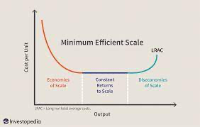
3.3 - Long-Run Production Costs
In the long run, all inputs are variable, which is where the firms aims to adjust to minimise costs regardless of what short run average total cost curve it is on.
Long run average total cost (LRATC) : same as short run ATC, but bigger
Economies of scale : LRATC declines as output increases
Diseconomies of scale : LRATC increaess as output increases
Constant returns to scale : output increase directly in proportion to an increase in all inputs (ex. input doubles, output also doubles)
3.4 - Types of Profit
As we know, there are concepts such as revenue, gains, and costs, which are all different than profit. Profit is the excess revenue that a business gets to keep.
Economic profit : revenue - explicit cost - implicit cost, or accounting profit - implicit cost
Accounting profit : revenue - explicit cost
Implicit cost : not an actual cost, a cost that you could’ve been earning (ex. if you own a restaurant, the implicit cost would be the salary you would have earned as being a chef working in a different restaurant)
Marginal Revenue: additional revenue gained by producing one more unit
3.5 - Profit Maximisation
The profit Maximising point for a firm is where it aims to increase revenue due to costs possibly being high as well.
MR = MC
If you cannot have MR=MC, MR>MC
The firms aim to produce where MR = MC due to the fact that all profits are earned without overshooting and gathering additional costs.
These calculations help a firm understand how much it must produce in order to maximise their profits.
3.6 - Firm’s’ Short-Run Decision to Produce and Long-Run Decisions to Enter or Exit a Market
Firms need to be able to know when to enter the market, as well as when to end production (entry and exit). By understanding profits, we are able to know what a firm does and therefore how many quantities to produce.
Short Run:
Shutdown rule : as long as P > AVC, continue to produce
If AVC > P : shutdown
Firms can make profit or losses
Long Run :
Exit rule : if P < ATC, exit the market
Firms make normal profit ($0), unless monopoly or oligopoly
Shut down rule: a firm should not produce unless it can cover its variable costs. If it is not able to do so, firms are better off producing nothing. However, this only tends to happen in perfect competition)
Perfect competition occurs when P<AVC at MR = MC)
As a result, this leads to long term adjustments in the long run where equalities in the market make a normal profit
3.7 Perfect Competition
In perfect competition, many identical firms are competing at a constant market price. This market has low barriers, meaning any firm is able to enter and exit the market in the long run.
Firms in this market are price takers, who are firms which cannot charge a higher price than the equilibrium price. This means that they have no market power.
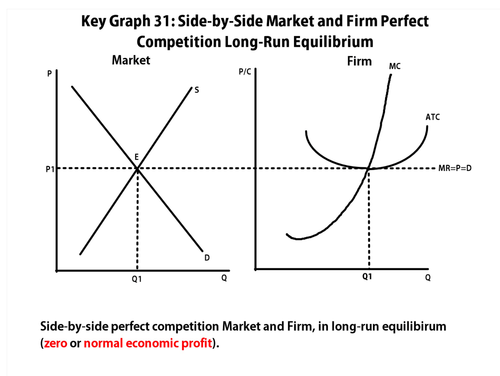
Long run will have normal profit
Short run can have either profit or loss