Factor demand

• The theory of factor demand is applicable to all factors of production but let’s focus on labor for now

Competitive factor markets

• Standard Assumptions

• Firms are price takers in the product market

• Firms are price takers in the input market

Marginal Revenue Product

• Demand for a unit of labor is a function of two things important to employers

1. Marginal productivity of the next unit of labor

• If total production could change greatly by the hiring of the next laborer, he/she would be beneficial for the firm

2. Firm must receive good value for the production

• This would be in the form of marginal revenue for the firm

• Marginal productivity of labor + marginal revenue = marginal revenue product of labor (MRPL)

• Change in total revenue/change in resource quantity = MR x MPl = P x MPl

• This is a measure of what a next unit of a resource (e.g. labor), brings to a firm

• Perfectly competitive output market, marginal revenue = price of the product

• From the chart of the same lemonade stand, we wouldn’t hire more than 1 worker because the marginal revenue product is maximized at that level

Profit-maximizing resource employment

• If MB > MC, do more of it

• If MB < MC, do less of it.

• If MB = MC, stop here.

• In the case of resource hiring, the marginal benefit is MRPL

• The marginal cost of resource hiring is marginal resource cost (MRC)

  • MRC is how much cost the firm incurs from using an additional unit of an input

  • In a competitive labor market, MRC = wage (w)

• MRC = Change in total resource cost/change in resource quantity = wage

• The profit-maximizing employer of labor would hire to the point where MRPL (marginal revenue product per labor)= MRC (marginal resource cost) = Wage

• Based on this chart, 3 workers would help maximize the profit for the lemonade stand MRPL as Demand for Labor

• Employment and labor cost are inversely related

• As labor cost increases, employment decreases, and vice versa

• Based on the same chart above, if the wage rate rose to $10, then the lemonade owner would have to cut down to 2 employees to maximize profit

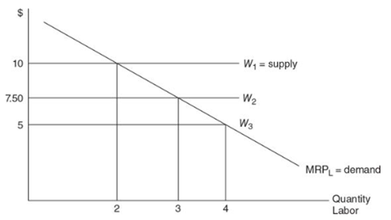
• MRPL is downward sloping like any demand curve would be, because of the diminishing marginal productivity of labor in the short run

• Demand for the overall market of labor is the sum of all of the individual firms’ MRPL curves: Market DL = SMRPL

Market wage as supply of labor

• Under the assumptions of a perfectly competitive labor market, the supply of labor to the individual firm

  • Is perfectly elastic

  • Equal to the wage

• Hence the firms could employ all of the workers they desire at the going market wage

• In competitive markets, MRPL is the firm’s downward-sloping labor demand curve

• In competitive markets, wage is the firm’s horizontal labor supply curve

Derived demand

• An increase in the demand for a resource means that at any wage, the firm wishes to employ more of that resource

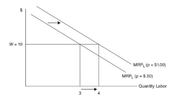
• ↑D for product leads to ↑price of product which ↑MRPL. This in return ↑hiring of labor at the current wage

Determinants of resource demand

1. Product demand

• Increase in demand for a product results in an increase in the price for that product

• Higher price increases the marginal revenue product of resources used in the production for that product

• Shifts the demand for those resources to the right and vice versa for opposite scenarios

2. Productivity (output per resource unit)

• If productivity increases, the firm takes advantage due to profit motives

• Productivity of a resource is affected by a few different factors

A. Quantity of other resources A.

• A good example would be how if the working space is improved or the labor is provided with better equipment, it can boost productivity

B. Technical progress

• Improvement in technology helps boost productivity greatly

C. Quality of variable resources

• Variable resources such as a well-trained work force can help boost productivity

• Prices of other resources

Demand for one (labor) often depends upon the prices of the others such as:

1. Substitute resources

A. Substitution effect (SE)

• As firms become more machinery dependent, they would obviously cut down on their labor

B. Output effect (OE)

• With lower machine costs, production cost declines which motivates firms to produce more

• With more output production, firms now need more labor too with the lower marginal cost of producing

C. Net effect of a lower price of capital depends upon the magnitude of each effect

• If SE > OE, demand for labor falls

• If OE > SE, the demand for labor increases

2. Complementary resources

• Lower-priced machinery makes it more affordable for the firm and at the same time requires more labor

• This situation would hold true only if the labor and machinery work in complement to each other

• A good example would be transport-related companies when they face increase costs in terms of fuel etc.

• Due to this increased cost, they would utilize lower vehicles and hence there would be fewer need for the extra driver now who doesn’t have to drive anything

Least-cost hiring of multiple inputs

• Producers find the best cost-minimizing combination of two inputs, given the prices and production constraint

• We use the consumer’s decision as a model for the producer’s decision

There are 2 connections between production and cost

1. You must produce Q* units of output. Now find the least-cost ($TC) way of doing so.

2. You can only spend $TC. Now find the highest level of output (Q*)

3. MPl/Pl = MPk/Pk

   1. This is the least cost rule and is used to find the combination

Imagine a situation

1. Input is $1 per unit

2. MPL = 100 and the MPK = 10 at the current level of labor and capital

3. Increasing spending on labor by $1 would increase output by 100 units

4. That one extra dollar is coming from you spending one dollar less on capital

   1. If MPL/PL > MPK/PK, the firm would likely increase spending on L and decrease spending on K

   2. Law of diminishing marginal returns predicts that as you increase L, MPL falls

   3. As you decrease K, MPK rises

Factor supply and market equilibrium

Supply of labor

• Price of labor increases, more hours of labor should be supplied (supply increases) Wage and Employment Determination

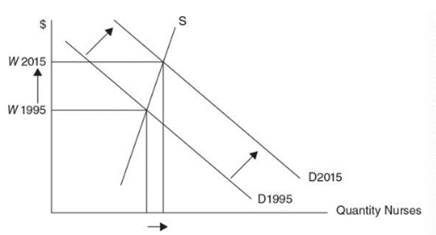
• Competitive wage is found at the intersection of labor demand and labor supply

What about Other Resources?

• The same concept would apply to even the market for capital

• Assuming that the market is in perfect competition

• MRPk = P x MPk

• Demand for capital is also derived from the marginal revenue product of capital (MRPK)

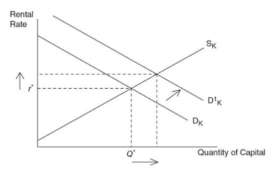
• The demand and supply operate as they normally do for any resource Imperfect Competition in Product and Factor Markets

Let’s assume that now the firms have some market power in

1. Product market

2. Factor (labor) market

   1. Since not the firms are the price setters, the price would exceeds marginal revenue

   2. This impacts the marginal revenue product function

   3. MR < P: MRPm = MR x MPl < MRP

   4. The result is that optimal amount of employment falls at all wages

   5. In simpler terms, the monopolist hires fewer resources

Market Power in Factor Markets

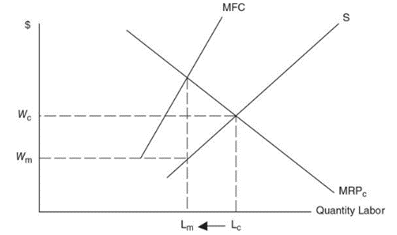
• Firms with extreme market power in the factor market are called wage-setting monopsonist

• The wages are set below marginal factor cost

Key difference between monopsony and perfectly competitive labor market is

1. Employer must increase the wage to increase the quantity of labor supplied

2. Labor supply to the firm is upward sloping

3. Marginal factor cost is now greater than the wage

• Considering the same lemonade stand, the stall owner can employ more workers by increasing wage but she would have to do the same for all existing employees

• Molly still chooses to employ where MRPL = MFC, but now wage is determined from the labor supply curve