Unit 2 - Supply and Demand Guide

All the basics of Supply and Demand which are the foundation of the majority of concepts moving forward.

2.1 - Demand

Demand: the quantity which a consumer/buyer are willing and able to buy at different prices
- Movement on the graph: downward sloping
- Demand slopes down on the graph due to:
  1. Income effect
  2. Substitution effect
  3. law of diminishing marginal utility
Law of Demand: As price increases, demand decreases, and as price decreases, demand increases
Determinants of demand:
- Taste and preferences, related goods, income, buyers, expectation of failure
Substitutes : good/service that can be used in place of another, when price of one increases, consumers will buy more of the other (ex. coffee and tea)
- Substitution effect: as the price of a good increases, consumers substitute the good with another that is cheaper
Complements : goods/services that are consumed together (ex. hamburgers and buns)
Income effect: as income increases, people will buy more of normal goods, and less of inferior goods
Normal good : increase in demand when consumer’s income increases (ex. oreos)
Inferior good : increase in demand when consumer’s income decreases (ex. off brand oreos)

Diminishing marginal utility: As more units of a product are consumed, the satisfaction/utility it provides tends to decline
- Apple users would purchase at maximum, a limited phones-they wouldn’t purchase a new iPhone every month since that extra phone would offer them no utility or not as much

Fig. 1 Demand curve

2.2 - Supply

Supply: different quantities of goods/services which sellers are willing and able to produce at a given price
Law of supply: as price increases, quantity supplied also increases, this is a direct relation.
The market supply shows the quantity a supplier is willing and able to offer at various prices at a given time

Reasons for the Law of Supply

Rising prices give greater opportunities to suppliers to earn a profit
With every additional unit, suppliers face an increase in the marginal cost of production
- Charging higher prices provides them with the easiest way to cover the cost
  - The vice versa is also true; lower prices wouldn’t provide the incentive to motivate the supplier and thus reduces the quantity of product
- The supply curve shifts upward, and the movement along the supply curve indicates a change in price.

Fig. 2 Supply Curve

Shifters of supply :
1. Resource costs and availability
  - The cost of production (land, labor, capital) has an inverse impact on the supply
  - When the cost of these increases, the supplier decides to produce less of the products since he is unable to afford the production cost
2. Other goods and services
  - Suppliers who produce more than one product (profit-maximizing firms) have an easier time switching to the production of another product if issues do arise in prices
  - E.g. A farmer has land where he is able to produce corn and earn a profit
  - If his land is capable to produce wheat as well, in case the price of wheat increases to that of corn, he would switch to wheat production to earn better
  - The supply curve in this situation for wheat would shift outwards(more supply) and vice versa for corn(reduced supply)
3. Technology
  - Newer technology causes the cost of production to decline and helps improve the efficiency of the supplier
  - This allows the supplier to produce more, shifting the supply curve outwards(toward right)
    - E.g. machines on the production line help reduce unit costs due to which more products are affordable by the supplier
4. Taxes and Subsidies
  - Taxes are added up to the unit cost of production, thus making it more expensive
  - Due to this, heavily taxed products are produced in less quantity by suppliers(supply curve shifts towards left)
  - Subsidies are the opposite of taxes and help reduce price per unit
  - This allows suppliers to produce more of the product(supply curve shifts towards the right)
5. Expectation
  - If suppliers expect prices to increase in the future, they would hold back supply for the current time with the future goal of earning more profit later (and vice versa)
6. Number of sellers
  - As the number of sellers increases in the market, the supply automatically increases
  - This allows consumers more choices at a lower price due to an increase in competition

2.3 - Price Elasticity of Demand

Equation : %∆Qd/%∆P
- 0 = perfectly elastic, <1 = inelastic, =1 unit elastic, >1 = elastic
Midpoint formula : Qd2-Qd1/(Q2d+Qd1)/2 , replace with Qd with price for price
Inelastic demand : TR correlates direct with price
Elastic demand = TR correlates inversely with price

Elasticity: how much the Q is affected by P.
- Elastic demand means that the goods are subject to be affected by a change in price.
- Inelastic demand means that goods are not subject to be affected by a change in price.

Characteristics of Elastic Demand:
- Flat, quantity is sensitive to price change, substitutes, luxury items, large portion of income, not needed immediately. Is equal to >1.
Characteristics of Inelastic Demand:
- Steep, few substitutes, required now, small portion of income, is equal to <1

Shapes of elasticity/inelasticity
- Perfectly elastic: infinity
- Relatively elastic: >1
- Unit elastic: 1
- Relatively inelastic: <1
- Perfectly inelastic: 0

2.4 - Price Elasticity of Supply

PES: measures how sensitive are sellers to price changes on goods
- Equation : %∆Qs/%∆P
- 0 = perfectly elastic, <1 = inelastic, =1 unit elastic, >1 = elastic
- Inelastic : unable to respond to price change
- Elastic : short run
- Extremely elastic : long run

Characteristics of inelastic Supply:
- Difficult production, high costs, hard to change to alternative, high barriers to entry, <1
Characteristics of Elastic Supply:
- Easy production, low cost, easy to switch to, low barriers to entry, >1

2.5 - Other Elasticities

Cross price elasticity of demand : %∆Qd of Good A/%∆P of good B
Negative = compliments (inferior good), positive = substitutes (normal good)
Income elasticity of demand : %∆Qd/%∆income
1 = income elastic, <1 = income inelastic, negative = inferior, positive = normal

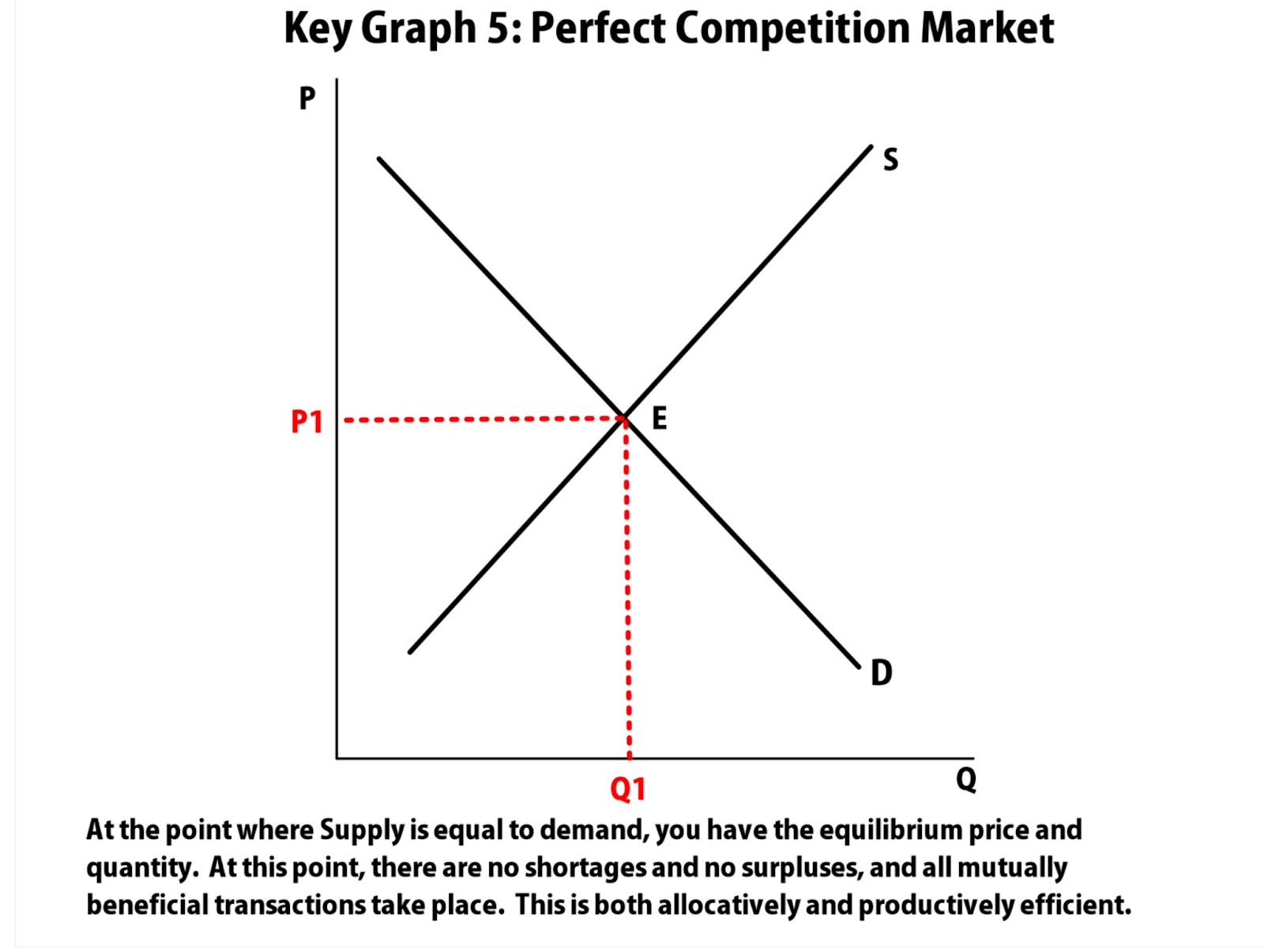
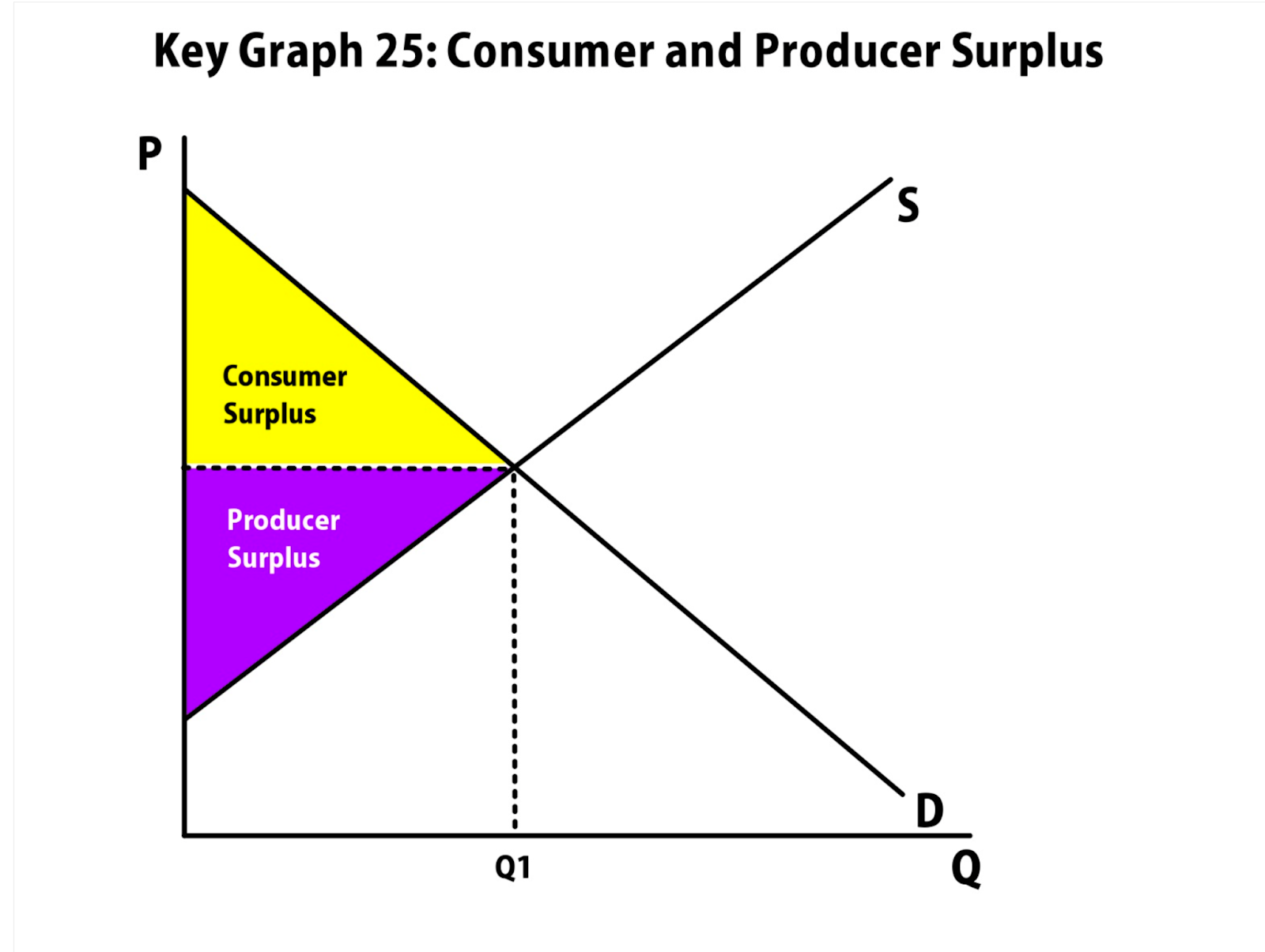
2.6 - Market Equilibrium, Consumer and Producer Surplus

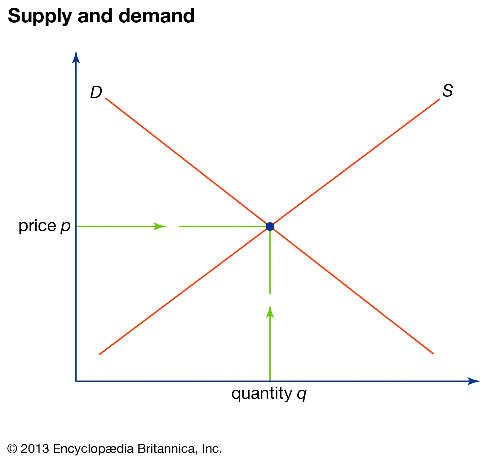
Equilibrium : occurs when no one is better off doing something else
- Equilibrium = Qs=Qd
- Price below the equilibrium is shortage
Consumer surplus : price consumers are willing to pay - actual price
Producer surplus : actual price -price the producer is willing to sell for

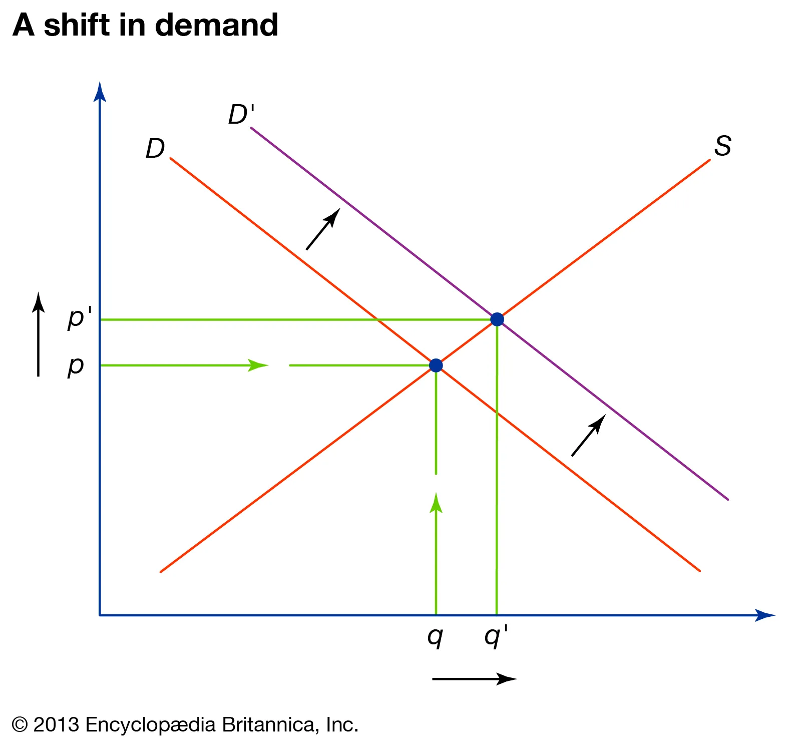
Fig. 4 Consumer and Producer Surplus

Demand increase : price and quantity increase
Demand decrease : price and quantity decrease

Supply increase : price decreases, quantity increases
Supply decrease : price increases, quantity decreases

Double shift : either price or quantity will be unknown. This rule states that when there is a simultaneous shift in both demand and supply, either price or quantity would stay indeterminate
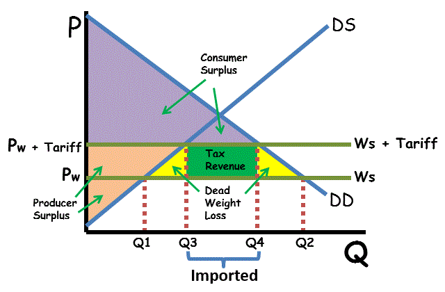
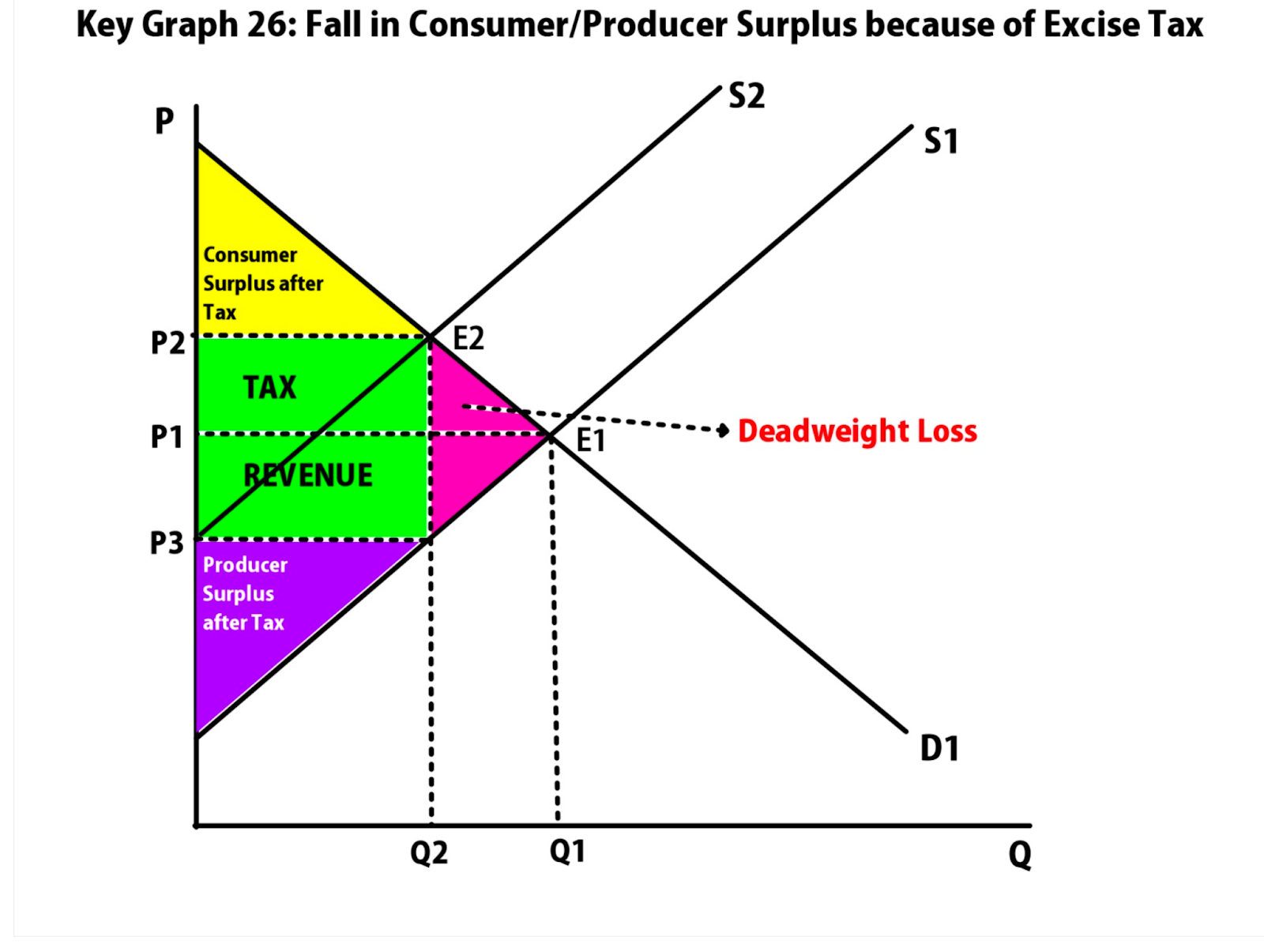
Deadweight loss (DWL) : transactions that should occur, but don’t because of government intervention (calculate the area = triangle formula, ½(base x height)

2.7 - Market Disequilibrium and Changes in Equilibrium

2.8 - Government Intervention in Markets

Market Disequilibrium:
- Shortage : Qs < Qd, price is lower than equilibrium
- Surplus : Qs > Qd, price is above equilibrium
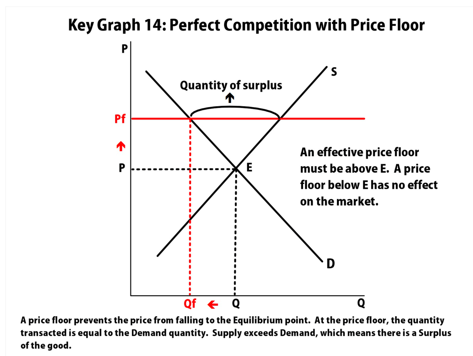
Price floor : minimum price a supplier can charge, price is set above equilibrium (causes shortage)
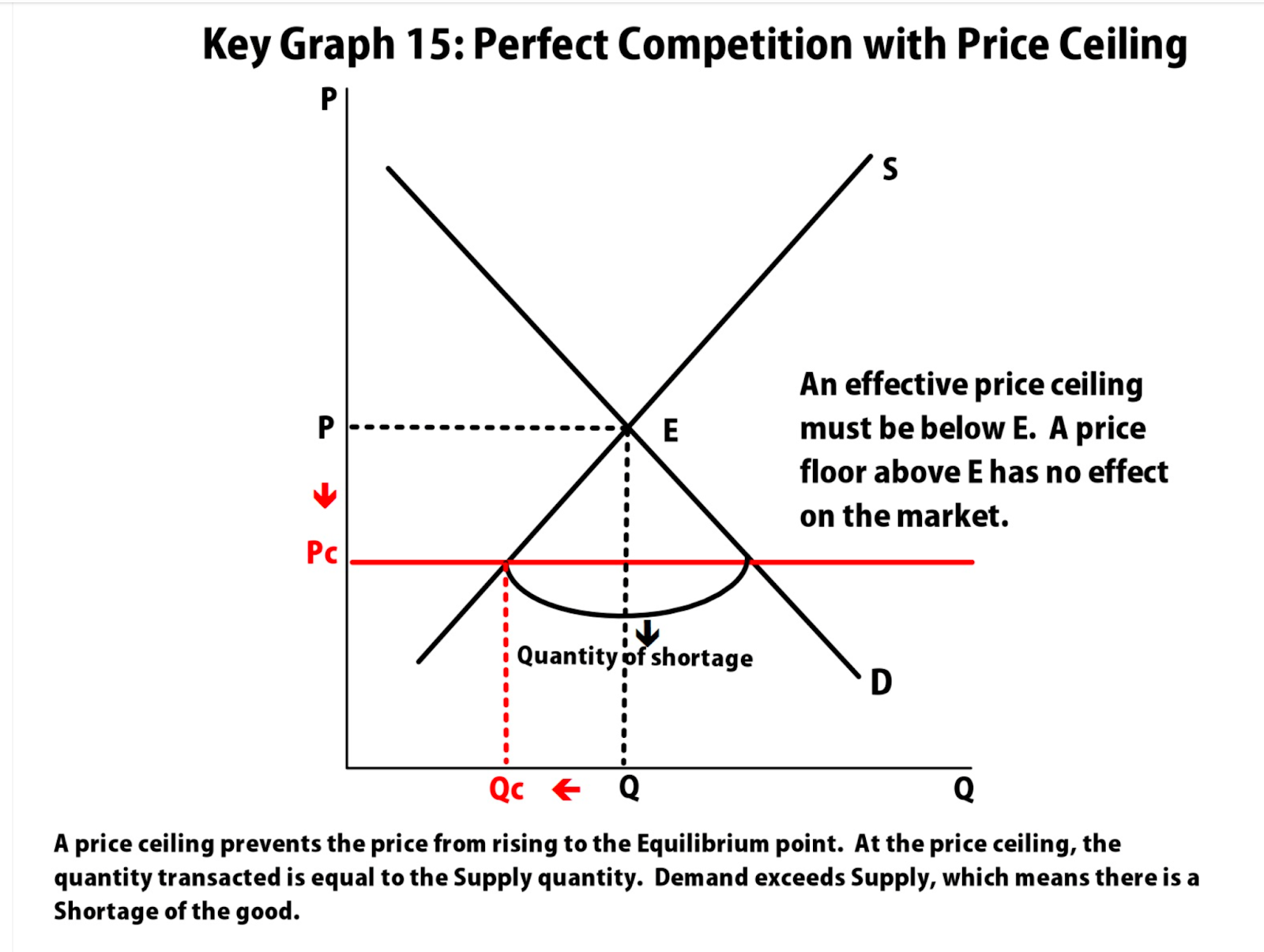
Price ceiling : maximum price a supplier can charge, price is set below equilibrium (causes surplus)
Quota : upper limit of a quantity that can be bought or sold (known as quantity control)
License : gives an owner the right to supply a good/service
Demand price : the price at which consumers will demand that quantity
Supply price : the price at which producers will supply that quantity

2.9 - International Trade and Public Policy

Quota rent : difference between demand price and supply price
Tariffs : tax placed on a good that is imported or exported
Import quota : restriction on the quantity of a good that can be imported

Fig. 8

Home

Business

AP Microeconomics

Unit 2: Supply and Demand