


Chapter 8: The Firm, Profit, and the Costs of Production
Profit and Cost: When CPAs and Economists Collide
Profit is different for an economist and an accountant
For an accountant, profit is total revenue – total cost
For an economist, would take into account the explicit and the implicit cost that was incurred as well
Implicit costs are the indirect, non-purchased opportunity cost that is incurred (also known as economic costs)
A good example would be when an entrepreneur opts for spending his savings, he is forgoing the interest he would have received if he were to deposit it into the bank
Explicit costs are the tangible business cost that arise such as the cash paid to suppliers, utility bills cost, etc.
Short-run and long-run decisions
Short run is referred to when at least one production input is fixed and cannot be changed due to a change in demand
A factory operating would be unable to increase the number of machinery in a short time if the demand increases suddenly
The long run is the opposite, where are production inputs are variable
The same factory would be able to increase its machinery to meet the demand after a period of a year for example after it would have generated sufficient profit to do so
Plant size (capital) | Fixed costs | Variable costs | Entry/exit of firms | |
|---|---|---|---|---|
Short run | fixed | Some | Some | No |
Long run | variable | None | All | Yes |
Short-run production functions
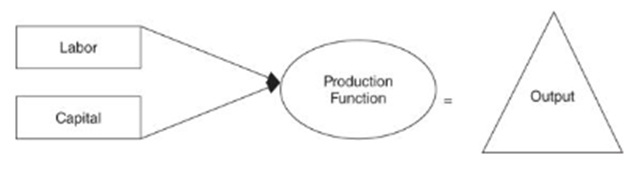
A production function is the mechanism for combining production resources with existing technology into finished goods and services
Fixed and variable inputs
Fixed inputs are those which can’t be altered in the short run for a business
Variable inputs are those which are easily alterable in the running of the business for the short run
If we consider the figure above, including only labor and capital, we could say that labor is a variable input while capital would be a fixed input
Short-run production measures
Total product of labor (TPL): this is the total quantity of output that is produced with each specific quantity of labor employed
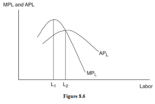
Marginal product of labor (MPL): this is the change in the total output if the quantity of labor is changed
Change in production output / Change in input labor
If labor is changing with one unit at a time, MPL = DTPL
Average product of labor (APL): this is used to measure the average labor productivity
TPL/L (total product produced by labor/ total labor)
Law of diminishing marginal returns
Unit of labor | Total product (TP) | Marginal product (MP) | Average product (AP) |
|---|---|---|---|
0 | 0 cups | ||
1 | 5 | 5-0 | 5 |
2 | 15 | 10 | 7.5 |
3 | 30 | 15 | 10 |
4 | 40 | 10 | 10 |
5 | 45 | 5 | 9 |
6 | 40 | -5 | 6.67 |
7 | 30 | -10 | 4.29 |

As the labor force is increased, the total product increases, reaches a peak, and then begins to decline
This is because the fixed resource has reached its limit and eventually the marginal product begins to decline- this is the law of diminishing marginal utility
Take an example of a pizza shop that has 2 chefs make pizzas
As the shop adds more employees, specialization occurs at a particular stage but afterward, there would be too many people and too little responsibility
The kitchen would become overcrowded and hence would case wastage
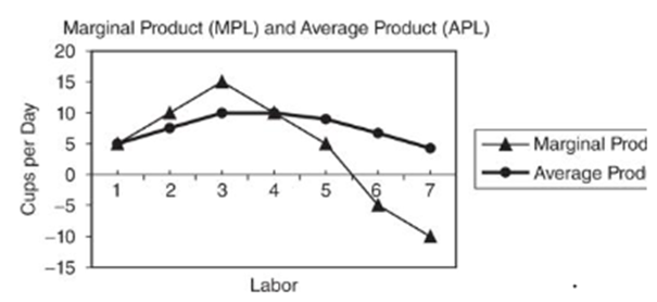
● MPL > APL: APL is rising ● MPL < APL: APL is falling ● MPL = APL: APL is at peak
Short-run costs
In the short run, at least one input is fixed
Hence due to this, fixed costs are incurred on it, while the other inputs which are variable incur their respective variable cost
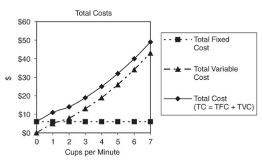
Total fixed costs (TFC): those costs that are incurred and have to be paid regardless of whether the company earns a profit or not
These costs are incurred regardless of whether the company produces something or not. E.g. rent expense
Total variable costs (TVC): the cost which directly varies with the level of output
If the company doesn’t produce anything, the total variable cost is 0. The best example of this is utility bills
Total cost (TC): the sum of total fixed cost and total variable cost.
If level of output is 0, total cost is equals to fixed cost
Total cost = Total fixed cost + total variable cost
Other costs
1. Marginal cost:
The additional cost of producing one more unit of output
Change in total cost / change in quantity
Another formula is DTVC/DQ which is change in total variable cost/change in quantity
2. Average fixed cost (AFC):
AFC = TFC/Q
It’s the total fixed cost divided by output
3. Average variable cost (AVC):
It’s the total variable cost divided by output
AVC = TVC/Q
4. Average total cost (ATC):
It’s the total cost divided by the output
ATC = TC/Q
ATC = AFC + AVC
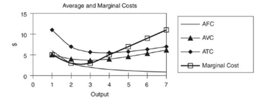
Marginal cost initially falls due to specialization but soon begins to rise as more output is produced
This is the law of increasing costs and is a direct result of the law of diminishing marginal returns to production
Marginal cost = average total cost at the minimum of ATC
Marginal cost = average variable cost at the minimum of AVC

Marginal product and marginal cost
As MPL is falling (diminishing marginal returns), MC is rising.
As MPL is rising (increasing marginal returns), MC is falling.
When MPL is highest, MC is lowest.
Average product and average variable cost
As APL is falling, AVC is rising.
As APL is rising, AVC is falling
When APL is highest, AVC is lowest

Long-run average cost

Suppose a business currently operates at SRAC1 (small scale) in the first year
In the Second year, the business now expands, and achieves SRAC2 (medium scale) but only if it manages to produce more than 100 units otherwise it wouldn’t be recommended
In the Third year, the business expands further, achieving SRAC3 (large scale)but only after selling more than 250 units
Finally in the fourth year, the business expands to grand scale, achieving SRAC4 but only after it manages to produce more than 400 units
Economies of scale

These are advantages of increased plant size and are seen on the downward part of the LRAC curve
Reasons for this
Labor and managerial specialization
Ability to purchase and use more efficient capital goods
Achieving minimum efficient scale which is the lowest point on the long-run average cost curve
Constant returns to scale occur when LRAC is constant over a variety of plant sizes
Diseconomies of scale are the rising part of the LRAC curve and can occur if a firm becomes too large
When firms grow in size they bring along certain diseconomies in the form of
Distant management
Worker alienation
Problems with communication and coordination
Another bridge between production and cost
If the firm doubles both labor and capital in the long run, and the output more than doubles (increases from one to four units), this is increasing returns to scale
During this time, the average total cost falls
If firms double their inputs again, and output exactly doubles, the firm has constant returns to scale in production
Average total cost stays the same
If firms double their inputs one last time, and output increases by less than double (not a desired outcome), we say that the firm has decreasing returns to scale in production
Average total cost increases
When all inputs are double and…. | Output increases by | We call this… | At the same time, LRAC is … | And we call this …. |
|---|---|---|---|---|
More than double | Increasing returns to production | falling | Economies of scale | |
Exactly double | Constant returns to scale in production | horizontal | Constant returns to scale | |
Less than double | Decreasing returns to scale in production | rising | Diseconomies of scale |