


Chapter 13: F Distribution and One-way Anova
Introductory
Analysis of Variance: For hypothesis tests comparing averages between more than two groups
13.1 One-Way ANOVA
ANOVA Test: determine the existence of a statistically significant difference among several group means.
Variances: helps determine if the means are equal or not
ANOVA Conditions
Each population from which a sample is taken is assumed to be normal.
All samples are randomly selected and independent.
The populations are assumed to have equal standard deviations (or variances).
The factor is a categorical variable.
The response is a numerical variable.
Ho: μ1 = μ2 = μ3 = ... = μk
Ha: At least two of the group means μ1, μ2, μ3, ..., μk are not equal. That is, μi ≠ μj for some i ≠ j.
The null hypothesis: is simply that all the group population means are the same.
The alternative hypothesis: is that at least one pair of means is different.
Ho is true: All means are the same; the differences are due to random variation.
Ho is NOT true: All means are not the same; the differences are too large to be due to random variation.
13.2 The F Distribution and the F-Ratio
F-distribution: theoretical distribution that compares two populations
There are two sets of degrees of freedom; one for the numerator and one for the denominator.
To calculate the F ratio, two estimates of the variance are made.
Variance between samples: An estimate of σ2 that is the variance of the sample means multiplied by n (when the sample sizes are the same.).
Variance within samples: An estimate of σ2 that is the average of the sample variances (also known as a pooled variance).
SSbetween: the sum of squares that represents the variation among the different samples
SSwithin: the sum of squares that represents the variation within samples that is due to chance.
MS means: "mean square."
MSbetween: is the variance between groups
MSwithin: is the variance within groups.
Calculation of Sum of Squares and Mean Square
k: the number of different groups
nj: the size of the jth group
sj: the sum of the values in the jth group
n: total number of all the values combined (total sample size: ∑nj)
x: one value→ ∑x = ∑sj
Sum of squares of all values from every group combined: ∑x2
Between-group variability: SStotal = ∑x2 – (∑𝑥2) / n
Total sum of squares: ∑*x^*2 – (∑𝑥)^2n / n
Explained variation: sum of squares representing variation among the different samples→ SSbetween = ∑[(𝑠𝑗)^2 / 𝑛𝑗]−(∑𝑠𝑗)^2 / 𝑛
Unexplained variation: sum of squares representing variation within samples due to chance→ 𝑆𝑆within = 𝑆𝑆total – 𝑆𝑆between
df**'s for different groups (df's for the numerator)**: df = k – 1
dfwithin = n – k*:* Equation for errors within samples (df's for the denominator)
MSbetween = 𝑆𝑆between / 𝑑𝑓between: Mean square (variance estimate) explained by the different groups
MSwithin = 𝑆𝑆within / 𝑑𝑓within: Mean square (variance estimate) that is due to chance (unexplained)
Null hypothesis is true: MSbetween and MSwithin should both estimate the same value.
The alternate hypothesis: at least two of the sample groups come from populations with different normal distributions.
The null hypothesis: all groups are samples from populations having the same normal distribution
F-Ratio or F Statistic
𝐹 = 𝑀𝑆between / 𝑀𝑆within
F**-Ratio Formula when the groups are the same size:** 𝐹 = 𝑛⋅𝑠𝑥^2 / 𝑠^2 pooled
where ...
n: the sample size
dfnumerator: k – 1
dfdenominator: n – k
s2 pooled: the mean of the sample variances (pooled variance)
sx¯^2: the variance of the sample means
13.2 Facts About the F Distribution
Here are some facts about the F distribution.
The curve is not symmetrical but skewed to the right.
There is a different curve for each set of dfs.
The F statistic is greater than or equal to zero.
As the degrees of freedom for the numerator and for the denominator get larger, the curve approximates the normal.
13.4 Test of Two Variances
In order to perform a F test of two variances, it is important that the following are true:
The populations from which the two samples are drawn are normally distributed.
The two populations are independent of each other.
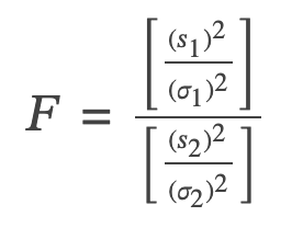
F has the distribution F ~ F(n1 – 1, n2 – 1)
where n1 – 1 are the degrees of freedom for the numerator and n2 – 1 are the degrees of freedom for the denominator.
F is close to one: the evidence favors the null hypothesis (the two population variances are equal)
F is much larger than one: then the evidence is against the null hypothesis
A test of two variances may be left, right, or two-tailed.
Examples