


Chapter 6: Two-Variable Data Analysis
In this chapter, we consider techniques of data analysis for two-variable (bivariate) quantitative data.
Scatterplots
It is a two-dimensional graph of ordered pairs.
We put one variable (explanatory variable) on the horizontal axis and the other (response variable) on the vertical axis.
The horizontal axis is considered to be independent, while the other is dependent.
The two variables are positively associated if higher than average values for one variable are generally paired with higher than average values of the other variable.
They are negatively associated if higher than average values for one variable tend to be paired with lower than average values of the other variable.
Correlation
Two variables are linearly related to the extent that their relationship can be modeled by a line.
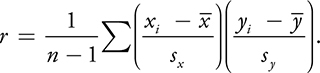
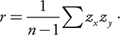
The first statistic we have to quantify a linear relationship is the Pearson product moment correlation, or, more simply, the Correlation Coefficient , denoted by the letter r .
It is a measure of the strength of the linear relationship between two variables as well as an indicator of the direction of the linear relationship.
For a sample of size n paired data (x,y), r is given by:
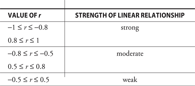
Properties of “r“
If r = −1 or r = 1, the points all lie on a line.
If r > 0, it indicates that the variables are positively associated.
if r<0, it indicates that the variables are negatively associated.
If r = 0, it indicates that there is no linear association that would allow us to predict y from x.
r depends only on the paired points, not the ordered pairs.
r does not depend on the units of measurement.
r is not resistant to extreme values because it is based on the mean.
Correlation and Causation
Just because two things seem to go together does not mean that one caused the other—some third variable may be influencing them both.
Linear Models
Least-Squares Regression Line
A line that can be used for predicting response values from explanatory values.
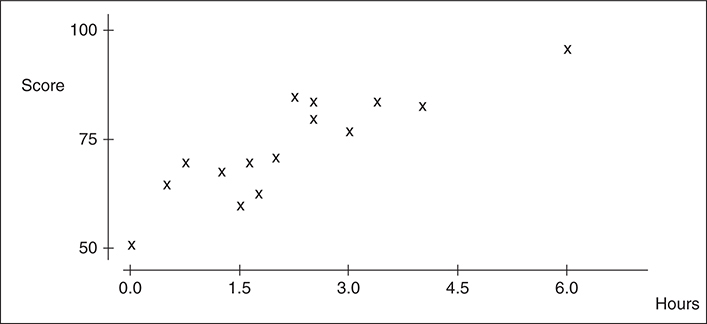
If we wanted to predict the score of a person that studied for 2.75 hours, we could use a regression line.
The least-squares regression line (LSRL) is the line that minimizes the sum of squared errors.
Let ŷ = predicted value of y for a given x
now (y-ŷ) = error in the prediction.
To reduce the errors in prediction, we try to minimize Σ(y-ŷ)^2.
Example:
Given below is the data from a study that looked at hours studied versus score on an exam:
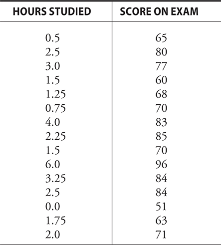
Here, ŷ = 59.03 + 6.77x
If we want to predict the score of someone that studied 2.75 hours, we plug this value into the above equation.
ŷ = 59.03 + 6.77(2.75)=77.63
Residuals
The formal name for (y - ŷ) is the residual.
Note that the order is always “actual” − “predicted”.
A positive residual means that the prediction was too small and a negative residual means that the prediction was too large.
If a line is an appropriate model, we would expect to find the residuals more or less randomly scattered about the average residual.
A pattern of residuals that does not appear to be more or less randomly distributed about 0 is evidence that a line is not a good model for the data.
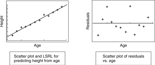
The line on the left is a good fit and the residuals on the right show no obvious pattern either. Thus the line is a good fit for the data.
Predicting a value of y from a value of x is called interpolation if we are predicting from an x-value within the range.
It is called extrapolation if we are predicting from a value of x outside of the x -values.
Coefficient of Determination
The Proportion of the total variability in y that is explained by the regression of y on x is called the coefficient of determination .
The coefficient of determination is symbolized by r^2.
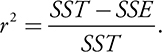
SST = sum of squares total. It represents the total error from using ȳ as the basis for predicting weight from height.
SSE = sum of squared errors. SSE represents the total error from using the LSRL.
SST − SSE represents the benefit of using the regression line rather than ȳ for prediction.
Outliers and Influential Observations
An outlier lies outside of the general pattern of the data.
An outlier can influence the correlation and may also exert an influence on the slope of the regression line.
An influential observation is one that has a strong influence on the regression model.
Often, the most influential points are extreme in the x -direction. We call these points high-leverage points.
Transformations to Achieve Linearity
There are many two-variable relationships that are nonlinear.
The path of an object thrown in the air is parabolic (quadratic).
Population tends to grow exponentially.
We can transform such data in such a way that the transformed data is well modeled by a line. This can be done by taking logs, or raising the variables to a power.
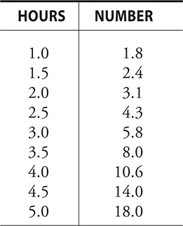
Example 1:
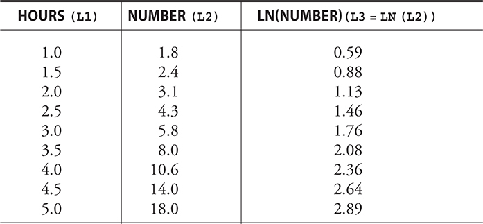
The number of a certain type of bacteria present somewhere after a certain number of hours given in the following chart. What would be the predicted quantity of bacteria after 3.75 hours?
Solution:
The scatterplot and residual plot for this data comes out as follows:
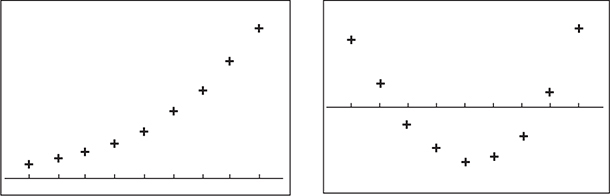
The line is NOT a good model for the data.
Now if we take log of the number of bacteria:
The scatterplot and residual plot for the new data comes out as follows:
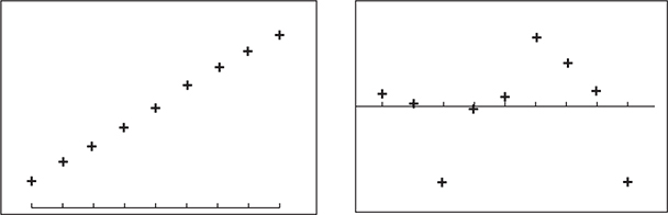
Now the scatterplot is more linear and the residual plot no longer has any distinct pattern.
The regression equation of the transformed data is:
ln(Number)=-0.047 + 0.586(Hours)
Therefore, after 3.75 hours,
ln(Number)=-0.047 + 0.586(3.75)=2.19.
Now to get back the original variable Number, we remove the log.
Number= e^2.19.
Example 2:
A researcher finds that the LSRL for predicting GPA based on average hours studied per week is
GPA = 1.75 + 0.11(hours studied). Interpret the slope of the regression line in the context of the problem.
Solution:
A student who studies an hour more than another
is predicted to have a GPA 0.11 points higher than the other student.
Example 3:
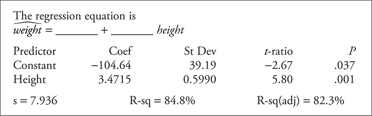
What is the regression equation for predicting weight from height in the following computer printout, and what is the correlation between height and weight?
Solution:
Weight = -104.64 + 3.4715(Height)
r^2 = 84.8% = 0.848.
r = 0.921.
As r is positive, the slope of the regression line is also positive.
Click the link to go to the next chapter: